Gradient Descent Simplified for Machine Learning Mastery!

Understanding of Gradient Descent algorithm is important for anyone who wants to gain deeper knowledge on how machine algorithms works. This is one of the fundamental mathematical tools which is common in basic machine learning models like linear regression to more advanced ones like neural networks.

➡ Definition
Gradient Descent is an iterative optimization algorithm used to minimize loss function in machine learning models. The main objective is to find the least possible error by iteratively adjusting parameter values.

➡ Building Blocks of Gradient Descent
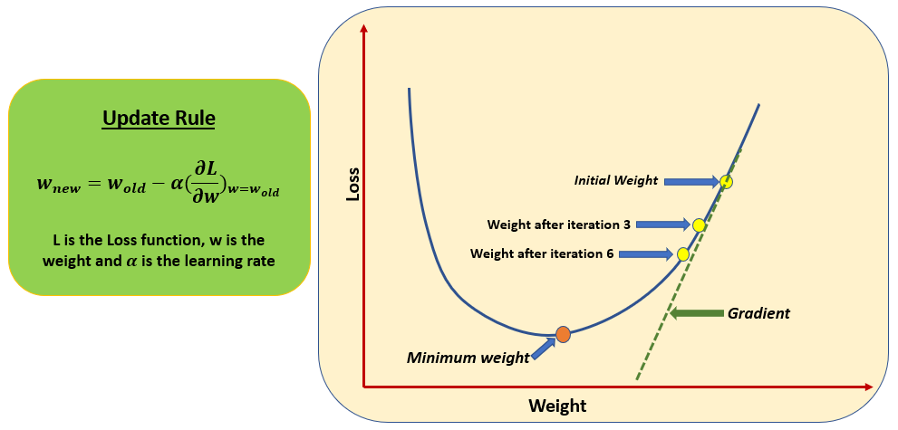
1. Loss Function: The loss function, also known as the cost function or objective function, measures the difference between predicted and actual values. It quantifies the error of the model's predictions.

2. Gradient: The gradient of the loss function represents the direction and magnitude of the steepest ascent. By taking steps in the opposite direction, we get steepest descent and reach the minimum of the loss function.

3. Learning Rate: The learning rate, often denoted as α, is a hyperparameter that determines the size of the steps taken during optimization. It controls the rate at which the model's parameters are updated.

4. Model Parameters: These are the variables within the model that are optimized during training. For example, in neural networks, the model parameters are the weights and biases.

➡ Primary usage of Gradient Descent in Machine Learning
1. Parameter Optimization
2. Model Training
3. Feature Selection

➡ Execution Steps of Gradient Descent
1. Begin by initializing model parameters (say weights and biases in neural networks) with random values.
2. Use the current parameter values to make predictions on the training data.
3. Use loss function to quantify the difference between actual and predicted values.
4. Compute the gradient of the loss function with respect to each parameter using partial differentiation.
5. Adjust parameters by taking steps in the opposite direction of the gradient. The magnitude of the update is determined by the learning rate.
6. Repeat steps 2-5 iteratively until convergence criteria are met (e.g. a predetermined number of iterations or a sufficiently small change in loss).

Did I miss something? Feel free to add in comments section.